Create a dropdown list with color in Excel and Google Sheets

Dropdowns are helpful options that simplify knowledge entry and implement knowledge validations in spreadsheet software program. Creating a dropdown list is straightforward. And also you might need finished that already in Excel or Google Sheets. However do you know, you can even assign a background color to your dropdown list objects? A coloured dropdown makes your knowledge simpler to learn and makes consumer picks simpler to determine. On this submit, we are going to present easy methods to create a dropdown list with color in Microsoft Excel and Google Sheets.

Should you use Microsoft Excel as your most well-liked analytic instrument, you would possibly already be acquainted with the idea known as conditional formatting. Conditional formatting, because the identify suggests, is used to format the content material of a cell primarily based on a sure situation. For instance, you could use conditional formatting to focus on duplicate cell values. In a comparable method, you could use conditional formatting to assign colours to objects in a dropdown list.

Equally, in case you use Google Sheets on a frequent foundation, you could already know easy methods to apply knowledge validation guidelines to cell values. These guidelines can be utilized to create a dropdown list, in addition to to assign colours to the dropdown list objects.

We have now beforehand coated easy methods to create a dropdown list in Microsoft Excel and Google Sheets. Within the following sections, we are going to see easy methods to color code dropdown lists in Microsoft Excel and Google Sheets.

How you can create a dropdown list with color in Excel

To create a color-coded dropdown list in Microsoft Excel, you first have to create a dropdown list and then you’ll be able to transfer forward so as to add colours to the list objects.

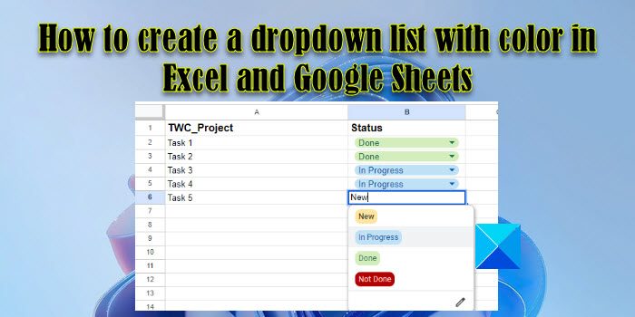
Allow us to say we now have a pattern spreadsheet as proven in the above picture whereby we now have a list of duties that must be marked as ‘New’, ‘In Progress’, ‘Done’, or ‘Not Done’. To take consumer enter, we are going to first create the dropdown list as follows:

• Choose cell B2.
• Go to the Knowledge tab.
• Choose Knowledge Validation from the Knowledge Instruments part.
• Choose List from the Enable dropdown.
• Sort ‘New,In Progress,Done,Not Done’ in the Supply area.
• Click on on the OK button.

The above steps will create a dropdown list subsequent to the primary activity in the spreadsheet. Subsequent, we are going to add colours to the dropdown list objects as follows:

• Choose cell B2.
• Go to the House tab.
• Click on on Conditional Formatting in the Types part.
• Choose New Rule from the dropdown that seems.
• Choose Format solely cells that include underneath Choose a Rule Sort.
• Underneath Format solely cells with, choose (and sort) Particular Textual content > containing > ‘New’, the place ‘New’ refers back to the merchandise in the list.
• Click on on the Format button.
• Within the Format Cells window, swap to the Fill tab.
• Choose the color that must be related with the dropdown list merchandise ‘New’. On this instance, we’re making use of a shade of yellow to the brand new duties assigned.
• Click on on the Okay button.
• Click on on the Okay button once more in the following window. Thus far, we now have related color with the list merchandise ‘New’.
• Repeat the method (steps 1 to 11) for different list objects – ‘In Progress’, ‘Done’, and ‘Not Done’, whereas making use of a completely different color to every of them. We have now utilized a shade of blue, a shade of inexperienced, and a shade of pink to those objects in this instance.
• Go to House > Conditional Formatting > Handle Guidelines to open the Conditional Formatting Guidelines Supervisor.
• Preview and confirm all the principles that you simply’ve utilized to the dropdown list objects and click on on OK. Now you may have a color-coded dropdown list in cell B2.
• Take the cursor to the bottom-right nook of cell B2.
• Because the cursor turns into a plus (+) image, click on and drag the cursor until cell B6. This motion will copy the cell content material and the corresponding formatting guidelines of cell B2 to the cell vary B3:B6 (the place we have to have the dropdown list).

How you can create a dropdown list with color in Google Sheets

Identical to Microsoft Excel, Google Sheets means that you can create a dropdown list with color-coded values. Nevertheless, creating a colorized dropdown list is far simpler in Google Sheets than in Excel. It’s because Google Sheets has added a new characteristic to assign background colours to objects whereas creating a dropdown list (this was earlier achieved utilizing conditional formatting, identical to in Excel).

Allow us to see easy methods to create the identical dropdown list (as defined in the above part) in Google Sheets.

• Place your cursor in cell B2.
• Go to Knowledge > Knowledge Validation. The Knowledge validation guidelines pane will open on the appropriate facet of the spreadsheet.
• Click on on the Add rule button.
• Choose the worth Dropdown underneath Standards. You will notice 2 choices. Rename Possibility 1 as ‘New’ and assign yellow color to the choice utilizing the Color dropdown.
• Rename Possibility 2 as ‘In Progress’ and assign blue color to the choice.
• Click on on the Add one other merchandise button twice so as to add 2 extra list choices.
• Rename the list objects as ‘Done’ and ‘Not Done’ and change their background colours to inexperienced and pink respectively.
• Click on on the Executed button to save lots of the rule. You now have a color-coded dropdown list in cell B2.
• Take the mouse pointer to the bottom-right nook of the cell and as turns into a plus image, click on and drag the cursor until cell B6. This may copy the info and knowledge validation rule of cell B2 in cells B3 by means of B6.

That is how one can create a dropdown list with color-coded knowledge in Excel and Google Sheets. I hope you discover this submit helpful.

Learn: How you can join Google Sheets with Microsoft Excel.

How you can create sure or no Dropdown list with color in Google Sheets?

Place the cursor on the cell the place the dropdown list ought to seem. Choose Knowledge > Knowledge validation. Click on on the Add rule button in the appropriate facet. Choose Dropdown in ‘Criteria’. Rename ‘Option 1’ as Sure. Rename ‘Option 2’ as No. Assign colours to the choices to present them an eye-catchy look. Click on on the Executed button.

How do I alter the color of a chosen worth in a dropdown?

In Microsoft Excel, choose the cell the place the dropdown is positioned. Go to House > Conditional Formatting > Handle Guidelines. Double-click on the specified color. Click on on the Format button in the following window. Select a completely different color and click on on OK. In Google Sheets, choose the dropdown and click on on the edit (pencil) button on the backside of the merchandise list. Choose the specified color utilizing the color choices accessible in the appropriate panel and click on on the Executed button.

Learn Subsequent: How you can add a Tooltip in Excel and Google Sheets.