

Many people use Microsoft Excel to calculate the finances or do some additions and subtractions. We additionally know that it helps Macros which helps us to automate our duties. An Excel sheet isn’t any stranger to us and doesn’t require any introduction. However what number of of you already know there’s a field referred to as Name Box in Excel sheet that we use every day?
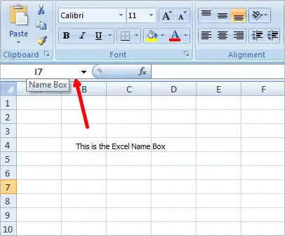
Sure, I’m speaking concerning the field on the prime left and beneath the ribbon. We typically suppose it’s simply the conventional field that provides reference to the energetic cell. However there’s a lot to learn about this, and we want to know the use of Excel Name Box.
What’s the Name Box perform in Microsoft Excel?
The Name Box perform in Microsoft Excel shows the cell at present chosen in the spreadsheet. It’s situated to the left of the method bar. If a reputation is outlined for a specific cell, the Name Box shows the title of the cell. You may use the Name Box to outline names for cells, ranges, constants, and formulation.
How to use Name Box in Excel
Makes use of of Name Box in Excel
I’ll take you thru some suggestions and methods that this Excel Name Box can implement.
Shortly go to the precise cell
If you’d like to go to a particular cell, then you’ll be able to kind the deal with of that cell in this Name Box. For instance, if you’d like to go to D10, then kind D10 into the Name Box, and that individual cell will get energetic.


Choose and Transfer to a particular vary of cells
If you’d like to choose and transfer to a particular vary of cells, then you’ll be able to use Excel Name Box. For instance, if you’d like to choose a variety from C8 to E13, you’ll be able to kind C8:E13 in the Name Box and hit Enter. Even if you’re at one other location, say Q10, you’ll return to the chosen vary as specified in the Excel Name Box.


Choose a selected vary from an energetic cell
If the energetic cell is B6 and also you kind C10 in the Name Box, press and maintain the Shift key of the keyboard and hit enter. You may see that vary B6:C10 will likely be chosen. Strive urgent and holding the Ctrl key, and also you see that solely cells B6 and C10 will likely be chosen and never the vary. Establish the distinction between them.


Choose A number of Specific Cells
Kind B4, E7, and G8 in the Name Box and hit enter. You see that each one three calls are chosen. You may attempt with A10, B17, and E5 and tell us. Word that the commas are used with none area.

Choose A number of Specific Ranges
Kind B4:C7 and E4:G7 in the Name Box and hit Enter. You see that two particular ranges, B4 via C7 and E4 via G7, bought chosen. Establish the colon and comma concerning the position.

To pick total Column(s)
Kind B:B in the Name Box and enter to see that the whole column B has been chosen. Strive typing B:E, and also you see that each one columns from B to E will likely be chosen utterly.

To pick total Rows(s)
Kind 3:3 in the Name Box, and you will notice that row 3 is chosen. Kind 3:6, and also you see that rows 3 via 6 are chosen. Do not forget that alphabets are to point out columns and numbers are to point out rows.

Choose a number of specific full rows
Beforehand, we noticed (in level 5) a tip to choose a number of specific vary cells. In the identical manner, we will choose a number of specific rows utilizing the Name Box. Kind 2:6,10:14 and hit enter. You see that rows 2 via 6 and 10 via 14 are chosen.

Collectively choose a number of specific total row(s) and column(s)
Kind G:G,7:7 in the Name Box and hit enter. You see that total column H and full row 7 have been chosen. In the identical manner, kind C:E,6:8, and hit enter. You see columns C via E and 6 via 8 get chosen collectively.

Choose intersection area of particular row(s) and column(s)
This offers the identical output as tip #2, however this time it identifies the area primarily based on the intersection of rows and columns you point out in the Name Box. For instance, we use the identical values talked about in tip #2. Kind C:E 8:13 in the Name Box and hit enter. You see that C8 to E13 will likely be chosen. Establish the area between E and eight.

Right here, the intersected space may be discovered by taking the primary column in the talked about vary ‘C’ and the primary row in the talked about vary ‘8’, and also you get the primary cell ‘C8’ of the intersection space. You’ll find the opposite cell worth of the intersection space.
Tip to choose the whole worksheet
Kind A:XFD in the Name Box and enter to see that the whole worksheet will likely be chosen.

Add one other chosen area to the already chosen area
Choose some area, say A2:D4 in the worksheet, and now kind E8:H12 in the Name Box. Now, press and maintain the Ctrl key on the keyboard and hit enter. You see, two ranges had been chosen A2 via D4 and E8 via H12. Strive Shift and see the enjoyable!

Choose the whole column and a row of an energetic cell
Choose any cell on the worksheet, kind ‘C’ in the Name Box, and hit enter. You see that the whole column of that energetic cell will get chosen. If you’d like to choose the whole row of the energetic cell, then kind ‘R’ in the Name Box and hit enter. This is likely one of the finest methods to say the use of Name Box in Excel, isn’t it?

Get again to the energetic cell by collapsing the chosen vary
Choose a variety on the worksheet and sort ‘RC’ in the Name Box. Hit enter, and also you see that you just get again to the energetic cell and the choice has collapsed.

Assign a reputation to the chosen vary
This tip exhibits you the use of Name Box in Excel. You may give a particular title to the chosen vary. Choose a variety on the worksheet and provides the title in the Name Box, and hit enter. You may use this title in place of the chosen vary in any method. This makes our job simpler in such case.

Later, if you’d like to choose the identical vary, you’ll be able to choose the title from the Name Box. Do not forget that title should have no areas in it.
These are some suggestions and methods for utilizing Name Box in Excel finest. I hope each tip will likely be helpful to some or the opposite to make your job easier. Strive a couple of extra with the assistance of those examples, and tell us. If you’d like to add something to this, please do share it with us via feedback.
Now see how to:
- Calculate the Sq. Root of the Quantity in Excel
- Cover System in Excel.
What’s the shortcut to Name a cell in Excel?
When naming a cell or vary in Excel, use the shortcut key Ctrl + F3 to open the Name Supervisor. Within the Name Supervisor, you’ll be able to create, edit, and delete any Excel names. As soon as a reputation is created, you’ll be able to use the shortcut key F3 to insert any title right into a cell.


