How to show Negative numbers in Red color in Google Sheets

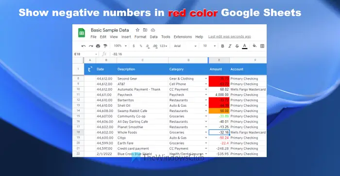
On this submit, we are going to assist you to show detrimental numbers in crimson color in a Google Sheets doc. This can come in helpful when you have got a dataset with values lower than 0 in totally different cells and also you need to spotlight them without delay to establish these values simply. The color of different values (having knowledge 0 or higher than 0) won’t change. Aside from that, each time you’ll replace the values (say altering the information from lower than 0 to a optimistic worth) in these cells, the color will change mechanically.

Show Negative numbers in Red color in Google Sheets doc

There are two other ways to spotlight detrimental numbers in crimson color in a Google Sheets doc. These are:

1. Utilizing Conditional Formatting
2. Utilizing Customized Formatting.

Let’s examine each the choices one after the other.

1] Spotlight detrimental numbers in crimson color in a Google Sheets doc utilizing Conditional Formatting

The conditional formatting possibility highlights all the cell with crimson color that has detrimental numbers. You can too select a customized color of your alternative to spotlight detrimental numbers. Let’s examine the steps:

1. Open a Google Sheets doc that comprises your dataset
2. Choose the cells having the detrimental numbers
3. Entry the Format menu
4. Click on on the Conditional formatting possibility. It’ll open the Conditional format guidelines field on the right-hand part
5. Click on on the drop-down menu obtainable for Format cells if… part
6. Choose the Lower than possibility from that drop-down menu
7. Enter 0 in the Worth or components field
8. Click on on the Fill color icon to open the color palette
9. Choose Red color from the palette. You can too select another color of your alternative
10. Press the Performed button.

That’s it. Now you’ll discover that each one the detrimental worth cells chosen by you’re highlighted with the crimson color or the color chosen by you. As you alter the values in the chosen cells, the color might be modified accordingly due to the rule set by you.

Additionally learn: How to change Date format in Google Sheets and Excel on-line.

2] Show detrimental numbers in crimson color in a Google Sheets doc utilizing Customized Formatting

Utilizing customized formatting, the color of chosen cells shouldn’t be modified, solely the worth color current in the chosen cells is modified in crimson color. You may’t set a customized color to spotlight detrimental numbers, solely crimson color is there. Listed here are the steps:

1. Open your Google Sheets doc that has your dataset
2. Choose the cells that embrace detrimental numbers
3. Click on on the Format menu of your Google Sheets doc
4. Entry the Quantity possibility
5. Click on on the Customized quantity format possibility current on the underside half. Customized quantity codecs field will pop-up
6. Within the Customized quantity format subject, paste Normal;[RED]Normal;Normal;@
7. Click on on the Apply button.

This can instantly spotlight detrimental values with crimson color in the cells chosen by you. Each time you’ll change the values in the cells the place you have got utilized the customized formatting, the color for detrimental values in these cells will change mechanically.

How do you spotlight detrimental numbers in crimson?

If you need to spotlight the detrimental numbers in crimson in a Google Sheets doc, then there are two methods for doing this. You should utilize the conditional formatting and customized formatting choices current beneath the Format menu of your Google Sheets doc. Whereas the primary possibility helps you to fill or spotlight the chosen cells (having detrimental numbers) with crimson color or a customized color, the latter possibility helps you to spotlight detrimental values in chosen cells with crimson color solely. We have now already lined each the choices individually with a step-by-step information in this submit above.

How do I color numbers in Google Sheets?

You should utilize the conditional formatting possibility obtainable beneath the Format menu of a Google Sheets doc to spotlight or color cells for the numbers or values. For instance, you’ll be able to set a rule that if the worth current in the chosen cell(s) is bigger than 10, then that cell might be crammed or highlighted with the inexperienced color or another color of your alternative.

Hope it’s useful for you.

Learn subsequent: How to add a picture in Google Sheets.