

It’s commonplace to discover duplicates whereas working with spreadsheets carrying giant information units. Although it might not be obligatory to take away every duplicate, discovering them manually for evaluation could possibly be a activity in itself. Excel supplies a straightforward manner to discover duplicates with conditional formatting. Google Sheets doesn’t present such an choice at current; nonetheless, it’s nonetheless doable to spotlight duplicates in it utilizing a customized formulation and a few conditional formatting guidelines.
On this article, we’re going to present you ways to spotlight duplicates in Google Sheets in the next methods:
- Highlight duplicate cells in a single column in Google Sheets.
- Highlight your entire row if duplicates are in one Google Sheets column.
- Highlight duplicate cells in a number of Google Sheets columns.
- Highlight precise duplicates, leaving the first occasion.
- Highlight full row duplicates in Google Sheets.
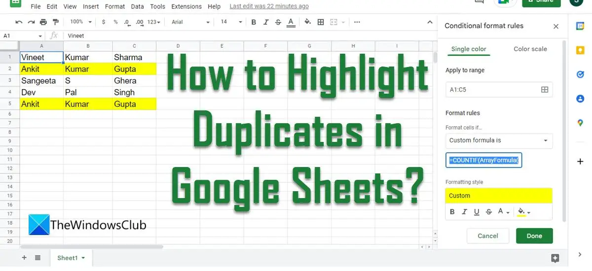
How to Highlight Duplicates in Google Sheets?
We’re going to use the COUNTIF operate to spotlight duplicates in Google Sheets. The COUNTIF operate counts throughout columns, row-by-row. The syntax of the COUNTIF operate is:
f(x)=COUNTIF(vary, criterion)
The place vary refers to the cell vary on which the operate wants to be utilized and criterion refers to the situation which wants to be met. The COUNTIF operate returns TRUE or FALSE based mostly on the match.
Now let’s see how the formulation works in Google Sheets.
1] Highlight duplicate cells in a single column in Google Sheets
Let’s say we’ve a spreadsheet with some names written in it. The sheet comprises some duplicate identify entries which we’re going to discover and spotlight utilizing the COUNTIF operate and conditional formatting in Google Sheets.
Open the spreadsheet you want to to work on. Click on on the Format menu on high of the spreadsheet. Choose Conditional formatting.


You’ll see the Conditional format guidelines panel on the proper aspect of the display screen. Click on on the icon subsequent to the Apply to vary choice and use your mouse pointer to choose a knowledge vary. For the dataset proven in the above picture, we’ve set the vary to A1:A10.


Choose Customized formulation is beneath the Format guidelines dropdown and enter the COUNTIF operate in the worth or formulation textbox.


We have now used the next formulation for the above dataset:
f(x)=COUNTIF($A$1:$A$10,$A1)>1
On this formulation, the situation has been set as $A1. The $ signal locks a column/row and tells the formulation to depend cells solely from the desired column/ row. So the $ signal right here signifies that the situation is predicated on column A solely. This can decide a cell worth from column A (A1, A2, and so forth), match it with all different cell values in column A and return True if a match is discovered. By including >1, we’re additional highlighting all of the cases of duplicates discovered inside column A.
By default, the cells might be highlighted in a shade shut to mild blue. You’ll be able to choose customized colours beneath the Formatting type choice to spotlight cells in the colour of your selection. We have now highlighted duplicates in yellow colour in our instance.


Click on on the Completed button to shut the Conditional format guidelines panel.
2] Highlight your entire row if duplicates are in one Google Sheets column

Utilizing the identical formulation, we are able to spotlight your entire row if duplicates are in one Google Sheets column. The one change right here can be the chosen vary (Apply to vary). We have now chosen A1:C10 right here, so conditional formatting will spotlight your entire row, as an alternative of highlighting particular person cells.
Additionally Learn: How to depend checkboxes in Google Sheets.
3] Highlight duplicate cells in a number of Google Sheets columns


We will regulate the identical formulation to spotlight duplicate cells in a number of Google Sheets columns. We’re making the next 2 adjustments to the formulation:
- Modifying the vary to cowl all information columns.
- Eradicating the $ signal from the criterion.
After eradicating the $ signal, the formulation will depend cells from all of the columns, together with columns A, B, C, and so forth. For the dataset proven in the above picture, the formulation might be:
f(x)=COUNTIF($A$1:$C$5,A1)>1
4] Highlight precise duplicates, leaving the first occasion


Once more, we are able to use the identical formulation to spotlight precise duplicates by ignoring the first occasion. For this, we’d like to lock the column in the tip vary, however not the row. On this association, every row will search for duplicates in its above rows solely.
For the dataset proven in the above instance, we’ve used the next formulation:
f(x)=COUNTIF($A$1:$A1,$A1)>1
5] Highlight full row duplicates in Google Sheets


We will use ArrayFormula with COUNTIF to spotlight full row duplicates in Google Sheets. ArrayFormula concatenates the information in a number of columns in a single string earlier than making use of the COUNTIF rule.
So for the above dataset, the operate might be:
f(x)=COUNTIF(ArrayFormula($A$1:$A$5&$B$1:$B$5&$C$1:$C$5),$A1&$B1&$C1)>1
This sums up other ways of highlighting duplicate cells in Google Sheets. Hope you discover this handy.
How do I discover duplicates in Google Sheets?
Google Sheets gives versatile methods to discover, evaluation or repair duplicate information. For instance, you may spotlight a single cell carrying the duplicate worth, or your entire row of knowledge if there’s a replica in a specific column. Duplicates could be highlighted based mostly on a situation and conditional formatting guidelines. The situation could also be outlined utilizing a customized formulation, resembling COUNTIF. Refer to the above article to find out how to use the COUNTIF operate in Google Sheets.
How do I spotlight duplicates in columns?
Suppose we’ve a spreadsheet containing information in the cell vary A1:C5. To focus on duplicates in a number of columns in this dataset, we might use the COUNTIF operate as, f(x)=COUNTIF($A$1:$C$5,A1)>1. This can decide a cell in a column, evaluate it with the remainder of the cells and return TRUE if a match is discovered. The comparability will occur for every column in the dataset.
How do I edit a rule in conditional formatting?
Comply with the steps to edit a rule in conditional formatting in Google Sheets:
- Choose the cell vary on which the rule has been utilized.
- Go to Format > Conditional formatting.
- Click on on the rule in the Conditional formatting rule pane on the proper aspect of the spreadsheet.
- Edit the formulation or formatting type as required.
- Click on on the Completed button.
To use one other rule on the identical vary, it’s possible you’ll use the ‘Add another rule’ choice. To delete a rule, you may click on on the trash icon subsequent to the rule.
Learn Subsequent: How to set up Customized Fonts on Google Docs.


