

Microsoft Excel is an software utilized by many all over the world, particularly for knowledge evaluation, due to the mathematical and statistical options it gives. On this tutorial, we are going to clarify how to highlight a cell or row with a test field in Excel.
How to highlight Cell or Row with Checkbox in Excel
To highlight a cell or row in Excel, we might be utilizing Conditional Formatting. The Conditional Formatting function simply spots, developments and patterns in your knowledge utilizing bars, colours, and Icons to visually highlight essential values. Comply with the steps under on how to highlight a cell or row with a test field in Excel:
- Launch Excel, then enter knowledge.
- Choose a cell.
- On the Developer tab, click on the Insert button in the Controls group, then click on the test field from the Type Controls group in the menu.
- Draw the test field into the chosen cell.
- Proper-click and choose Edit Textual content from the menu to take away textual content from the test field.
- Proper-click the test field button and choose Format Management
- Within the cell hyperlink field, kind the cell the place you need to hyperlink to the test field.
- Highlight the cell the place you need to add the conditional formatting to when the test field is chosen.
- Within the Choose a rule kind listing, choose ‘Use a formula to determine which cells to format.’
- Within the ‘Format value where this formula is true’ field, kind the cell the place you could have linked the checkbox to and add TRUE, for instance:
= IF ($E3=TRUE,TRUE,FALSE) - Click on the Format button, choose the Fill tab, and select a colour after which click on OK
- Click on each test containers to see the chosen rows highlighted.
Launch Excel.
Enter your knowledge.
Now we’re going to insert the test containers.
Choose a cell.


On the Developer tab, click on the Insert button in the Controls group, then click on the Verify Field from the Type Controls group in the menu.
Now draw the test field into the chosen cell.
In order for you to take away the textual content from the test field, right-click and choose Edit Textual content from the menu.
Now delete the textual content.


Proper-click the test field button and choose Format Management from the menu.
A Format Management dialog field will open.
Within the cell hyperlink field, kind the cell the place you need to hyperlink to the test field, for instance, $E3, then click on OK.
Now we’re going to add the conditional formatting to the cell.
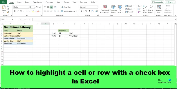
Highlight the cell the place you need to add the conditional formatting when the test field is chosen, for example, in the photograph, we’ve got highlighted a row containing Employees.


On the Residence tab, click on the Conditional Formatting button in the Types group, then choose New Rule from the menu.
A New Formatting Rule dialog field will open.


Within the Choose a rule kind listing, choose ‘Use a formula to determine which cells to format.’
Within the ‘Format value where this formula is true’ field, kind the cell the place you could have linked the test field, and add TRUE, for instance, = IF ($E3=TRUE,TRUE,FALSE).
Now we would like to choose a colour.
Click on the Format button, choose the Fill tab, and select a colour.
Then click on OK for each dialog containers.
Comply with the identical methodology for the opposite cells that you really want to highlight, with that colour, for example, in the photograph above, highlight all of the rows containing Employees.
On this tutorial, we would like the rows containing ‘Volunteer’ to have a special colour.
Proper-click the test field button adjoining to the cell containing ‘Volunteer’ and choose Format Management from the menu.

Within the cell hyperlink field, kind the cell the place you need to hyperlink to the test field, for instance, $E4, then click on OK.

Highlight the row the place you need to add the conditional formatting when the test field is chosen, for example, in the photograph, we’ve got highlighted a row containing ‘Volunteer.’
On the Residence tab, click on the Conditional Formatting button in the Types group, then choose New Rule from the menu.
A New Formatting Rule dialog field will open.

Within the Choose a rule kind listing, choose ‘Use a formula to determine which cells to format.’
Within the ‘Format value where this formula is true’ field, kind the cell the place you could have linked the checkbox and add TRUE, for instance, = IF ($E4=TRUE,TRUE,FALSE).
Now we would like to choose a colour.
Click on the Format button, choose the Fill tab, and select a colour.
Do the identical steps for the rows you need to highlight.

On this tutorial, you’ll discover that when the test field for Employees is chosen, the row containing ‘Staff’ is highlighted in pink, and when the test field for ‘Volunteer’ is checked, the colour of the row containing ‘Volunteer’ will flip blue.
How do I modify the looks of a checkbox in Excel?
- Proper-click the test field and choose Format Management from the menu.
- A Format Management dialog field will open.
- Click on the Colours and Strains tab. Then select a colour underneath the Fill part.
- You can too change the traces and the type of the test field.
- Then click on OK.
- The looks of the test field will change.
READ: How to add Border in Excel
How do I add a checkbox in Excel with out the Developer tab?
- Click on the Insert tab, click on the Image button drop-down, and choose Image.
- Within the dialog field, choose the font Winding, seek for the test field image, then click on OK.
- The image test field can’t be formatted just like the Developer test field; it’s only a image.
READ: How to add Alt Textual content in Excel
We hope you perceive how to highlight a cell or row with a test field in Excel.


