

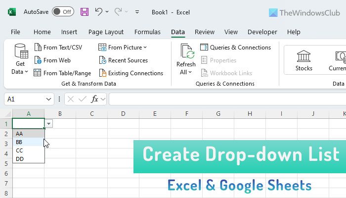
In case you are creating an interactive spreadsheet, it’s possible you’ll want a drop-down list in order that customers can select between choices. For that, you may comply with this tutorial to create a drop-down list in Microsoft Excel or Google Sheets. You’ll be able to create a single in addition to a nested drop-down menu with the assistance of this information.
Like varied programming languages, it’s attainable to embrace the if-else assertion in an Excel spreadsheet as nicely. Let’s assume that you’re creating a spreadsheet for individuals who ought to choose totally different choices in accordance to varied standards. At such a second, it’s smart to use a drop-down list so as to present multiple selection to the individuals.
How to create a drop-down list in Excel
To create a drop-down list in Excel, comply with these steps-
- Choose a cell the place you need to present the drop-down menu.
- Go to Information > Information Validation.
- Choose the List from the Permit menu.
- Write down your choices in the Supply field.
- Save your change.
To get began, you want to choose a cell in your spreadsheet the place you need to present the drop-down list. After that, change from the Dwelling tab to the Information tab. Within the Information Instruments part, click on the Information Validation button, and choose the identical possibility once more.


Now, broaden the Permit drop-down list, and choose List. Then, you want to write down all of the choices one after one. If you’d like to show AA, BB, and CC because the examples, you want to write them like this-
AA,BB,CC


Regardless of what number of choices you need to present, you want to separate them by a comma. After doing that, click on the OK button. Now, you must discover a drop-down list like this-

You’ll be able to add an error message as nicely. It seems when customers attempt to enter a totally different worth apart from the given choices. For that, change to the Error Alert tab, and write down your message. Observe this tutorial to add error messages in Excel.
How to create a nested drop-down list in Excel
If you’d like to get hold of knowledge from some current drop-down menus or cells and show choices accordingly in a totally different cell, here’s what you are able to do.
You want to open the identical Information Validation window and choose List in the Permit menu. This time, you want to enter a vary in the Supply field like this-
=$A$1:$A$5

In accordance to this vary, the brand new drop-down list will present the identical choices which are written in the A1 to A5 cells.
How to create a drop-down list in Google Sheets
To create a drop-down list in Google Sheets, comply with these steps-
- Choose a cell and go to Information > Information validation.
- Choose the List of things.
- Write down your objects or choices.
- Save your change.
First, choose a cell in a spreadsheet and click on the Information from the highest navigation bar. After that, choose the Information validation possibility from the list.


Now, broaden the Standards drop-down menu, and choose List of things. Subsequent, you want to write down all of the choices or objects in the empty field.

Ultimately, click on the Save button to present the drop-down list in a cell.
Like Excel, Google Sheets reveals a warning or error message for getting into invalid knowledge. By default, it reveals a warning message and permits customers to write customized textual content. If you’d like to stop customers from getting into invalid knowledge, you want to select the Reject enter possibility in the Information validation window.
That’s all! I hope it helps you.
Learn: How to convert and open Apple Numbers file in Excel on Home windows PC
How to create a nested drop-down list in Google Sheets


It’s nearly the identical as Excel, however the title of the choice is totally different. You want to choose the List from a vary possibility from the Standards list and enter a vary in accordance to your wants. You’ll be able to enter a subject like this-
=$A$1:$A$5
It’ll present all of the texts from A1 to A5 cells in this drop-down list. As you’ve gotten already guessed, you want to refill all these chosen cells first to present the choices. By selecting this feature, you’re locking customers to select solely from the chosen cells.
Learn: How to insert A number of Clean Rows in Excel without delay


