

Ratio is the comparability of two portions and is expressed by a colon (:). For instance, if the ratio of Class 1 and Class 2 in a faculty is 2:1, it represents that the variety of college students in Class 1 is twice the variety of college students in Class 2 in that college. This text exhibits how to calculate Ratios in Excel. There could also be some instances when you will have to signify information in Excel in the type of a ratio. This text will present you the way to try this.
How to calculate Ratio in Excel
We are going to present you the next two strategies to calculate the Ratio in Excel:
- By utilizing the GCD operate
- By utilizing the SUBSTITUTE and TEXT features
Let’s begin.
1] Calculate ratio in Excel by utilizing the GCD operate
GCD stands for Best Widespread Divisor. It’s also referred to as HCF (Highest Widespread Issue). In easy phrases, it’s the biggest quantity that may divide a selected set of numbers. For instance, the Best Widespread Divisor of the set of numbers 8, 12, and 20 is 4, as 4 can divide all these three numbers.


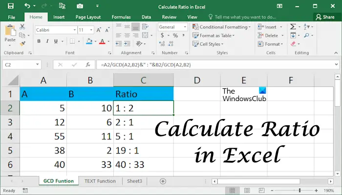
We are going to use this GCD operate in Excel to calculate the ratio. We’ve got created a pattern information proven in the above screenshot. First, we’ll calculate the GCD, then we’ll use this GCD worth to calculate the ratio.
Choose the cell in which you need to show the GCD. In our case, it’s the cell C2. Now, kind the next components and hit Enter.
=GCD(first worth,second worth)

Within the above components, change the primary worth and second worth with the cell numbers. For instance, in our case, the components seems to be like:
=GCD(A2,B2)

Enter the proper cell quantity, in any other case, you’ll get an incorrect consequence or an error. Now, copy your complete components to the remaining cells utilizing the Fill Deal with.
Now, we’ll use this GCD worth to calculate and show the ratio in our focused cells. Use the next components to calculate and show the ratio in Excel.
=first worth/GCD&" : "&second worth/GCD

Within the above components, we have now divided the primary and the second values by GCD and separated each of those values with the colon (:). In our case, the components seems to be like this:
=A2/C2&" : "&B2/C2

Within the above components, A2 is the cell containing the primary worth, B2 is the cell containing the second worth, and C2 is the cell containing GCD. Now, copy the components to the remaining cells utilizing the Fill Deal with function.
You’ll be able to immediately use the GCD components in the ratio components as a substitute of calculating and displaying the GCD values individually. For instance, in the next components, you will have to change the GCD with the precise GCD components:
=first worth/GCD&" : "&second worth/GCD
Therefore, the components will develop into:
=first worth/GCD(first worth,second worth)&" : "&second worth/GCD(first worth,second worth)

Exchange the primary and second values in the above components with the proper cell numbers. In our case, the whole components seems to be like this:
=A2/GCD(A2,B2)&" : "&B2/GCD(A2,B2)
After making use of the components to one cell, copy it to the remaining cells by utilizing the Fill Deal with. That is how to calculate ratios in Excel utilizing the GCD operate. Beneath, we have now defined the strategy to calculate the ratio in Excel by utilizing the SUBSTITUTE and TEXT features.
Learn: How to calculate Median in Excel
2] Calculate ratio in Excel by utilizing the SUBSTITUTE and TEXT features
Right here, we’ll use the TEXT operate to show the consequence in a fraction, then we’ll change the fraction with the ratio by utilizing the SUBSTITUTE operate. Right here, we’ll take the identical pattern information to present you.
If we divide the worth in the cell A2 by the worth in the cell B2, the components is:
=A2/B2
It will show the consequence in decimal. Now, to present this consequence in fractions, we’ll use the TEXT operate. Therefore, the components turns into:
=TEXT(A2/B2,"####/####")

Within the above components, you possibly can enhance # to enhance the accuracy. For instance, if you’d like to present fractions for up to 5 digits, you should use 5 # symbols.

Now, we’ll create the components to change the “/” with “:” by utilizing the SUBSTITUTE operate. Therefore, the whole components will develop into:
=SUBSTITUTE(TEXT(A2/B2,"####/####"),"/",":")

You’ll be able to enhance the # symbols in the above components to enhance the accuracy relying on the variety of digits you will have. When you’re achieved, copy the components to the remaining cells by utilizing the Fill Deal with.
Within the above formulae, use the cell addresses appropriately, in any other case, you’ll get an error.
Learn: How to Calculate Easy Curiosity in Excel.
How do you enter a ratio worth in Excel?
There isn’t a direct method to present the consequence as a ratio in Excel. For this, you will have to use acceptable formulae. You too can show the consequence as a fraction after which convert that fraction worth right into a ratio.
What’s a ratio information in Excel?
The ratio information in Excel is the comparability of two values. For instance, worth 1 is what number of instances worth 2. There are other ways to calculate and present ratios in Excel. You need to use any of those strategies.
That’s it. I hope this helps.
Learn subsequent: Calculate the Weight to Top ratio and BMI in Excel utilizing this BMI calculation components.


